A worked example from the lecture notes of a course I taught entitled Advanced Computational Methods in Geotechnical Engineering. The finite difference and finite element methods both reduce a boundary value problem to a system of linear algebraic equations of the form \(\boldsymbol{A} \boldsymbol{x} = \boldsymbol{b}\). For the large, sparse systems that arise from fine discretizations, iterative solvers are often preferred over direct methods such as Gaussian elimination. This note develops the three classical stationary iterative methods, Jacobi, Gauss-Seidel and successive over-relaxation (SOR), and compares their convergence on a model problem.
Stationary Iterative Methods
A stationary iterative method is built from a splitting of the coefficient matrix,
\[\boldsymbol{A} = \boldsymbol{M} - \boldsymbol{N}\]which turns \(\boldsymbol{A}\boldsymbol{x} = \boldsymbol{b}\) into the fixed-point iteration
\[\boldsymbol{M} \boldsymbol{x}^{(k+1)} = \boldsymbol{N}\boldsymbol{x}^{(k)} + \boldsymbol{b} \qquad \Longrightarrow \qquad \boldsymbol{x}^{(k+1)} = \boldsymbol{M}^{-1}\boldsymbol{N}\,\boldsymbol{x}^{(k)} + \boldsymbol{M}^{-1}\boldsymbol{b}\]The iteration converges, for any starting vector, if and only if the spectral radius of the iteration matrix satisfies \(\rho(\boldsymbol{M}^{-1}\boldsymbol{N}) < 1\). The different methods correspond to different choices of \(\boldsymbol{M}\). It is convenient to decompose \(\boldsymbol{A}\) into its diagonal, strictly lower and strictly upper parts,
\[\boldsymbol{A} = \boldsymbol{D} + \boldsymbol{L} + \boldsymbol{U}\]Jacobi Method
The Jacobi method takes \(\boldsymbol{M} = \boldsymbol{D}\), so that every component is updated using only values from the previous iterate,
\[x_i^{(k+1)} = \frac{1}{a_{ii}} \left( b_i - \sum_{j \neq i} a_{ij}\, x_j^{(k)} \right)\]Gauss-Seidel Method
The Gauss-Seidel method takes \(\boldsymbol{M} = \boldsymbol{D} + \boldsymbol{L}\), reusing components as soon as they are updated within the same sweep,
\[x_i^{(k+1)} = \frac{1}{a_{ii}} \left( b_i - \sum_{j < i} a_{ij}\, x_j^{(k+1)} - \sum_{j > i} a_{ij}\, x_j^{(k)} \right)\]Because new information is used immediately, Gauss-Seidel typically converges about twice as fast as Jacobi for the problems considered here.
Successive Over-Relaxation
SOR accelerates Gauss-Seidel by extrapolating each update with a relaxation factor \(\omega \in (0,2)\),
\[x_i^{(k+1)} = (1-\omega)\, x_i^{(k)} + \frac{\omega}{a_{ii}} \left( b_i - \sum_{j < i} a_{ij}\, x_j^{(k+1)} - \sum_{j > i} a_{ij}\, x_j^{(k)} \right)\]Setting \(\omega = 1\) recovers Gauss-Seidel, \(\omega > 1\) is over-relaxation and \(\omega < 1\) is under-relaxation. For a consistently ordered, symmetric positive definite matrix the optimal factor can be obtained from the spectral radius of the Jacobi iteration matrix \(\rho_J\),
\[\omega_{\mathrm{opt}} = \frac{2}{1 + \sqrt{1 - \rho_J^2}}\]The iteration is run until the change between successive iterates falls below a prescribed tolerance, i.e. \(\lVert \boldsymbol{x}^{(k+1)} - \boldsymbol{x}^{(k)} \rVert \leq \varepsilon\).
A Model Problem
We consider the tridiagonal system used in the course assignment, where the coefficient matrix has \(-2\) on the main diagonal and \(1\) on the two off-diagonals, and the right hand side is \(\boldsymbol{b} = \{4, 0, 0, \cdots, 0\}^{\mathrm{T}}\),
\[\left[ \begin{matrix} -2 & 1 \\ 1 & -2 & 1 \\ & \ddots & \ddots & \ddots \\ & & 1 & -2 & 1 \\ & & & 1 & -2 \end{matrix} \right] \left\lbrace \begin{matrix} x_1 \\ x_2 \\ \vdots \\ x_{n-1} \\ x_n \end{matrix} \right\rbrace = \left\lbrace \begin{matrix} 4 \\ 0 \\ \vdots \\ 0 \\ 0 \end{matrix} \right\rbrace\]This matrix is the standard second-difference operator that appears, for example, when the finite difference method is applied to one-dimensional steady-state flow or consolidation. It is symmetric and weakly diagonally dominant, which guarantees that both the Jacobi and Gauss-Seidel iterations converge; SOR converges for any \(\omega \in (0,2)\).
Python Implementation
The three methods are implemented below using the matrix splitting directly. The same routine covers all three by passing the appropriate relaxation factor.
import numpy as np

def tridiag(n):
    A = np.zeros((n, n))
    np.fill_diagonal(A, -2.0)
    for i in range(n - 1):
        A[i, i + 1] = A[i + 1, i] = 1.0
    return A

def rhs(n):
    b = np.zeros(n)
    b[0] = 4.0
    return b

def stationary_solve(method, A, b, omega=1.0, tol=1e-11, maxit=1000):
    n = len(b)
    D = np.diag(np.diag(A))
    L = np.tril(A, -1)
    U = np.triu(A, 1)
    x = np.zeros(n)
    history = []
    for k in range(maxit):
        if method == "jacobi":
            x_new = np.linalg.solve(D, b - (L + U) @ x)
        elif method == "gauss_seidel":
            x_new = np.linalg.solve(D + L, b - U @ x)
        elif method == "sor":
            x_new = np.linalg.solve(D + omega * L,
                                    omega * b - (omega * U + (omega - 1.0) * D) @ x)
        history.append(np.linalg.norm(x_new - x))
        x = x_new
        if history[-1] < tol:
            break
    return x, history

# Optimal relaxation factor from the Jacobi spectral radius
def omega_opt(A):
    D = np.diag(np.diag(A))
    M_jacobi = -np.linalg.solve(D, A - D)
    rho = max(abs(np.linalg.eigvals(M_jacobi)))
    return 2.0 / (1.0 + np.sqrt(1.0 - rho ** 2))

A, b = tridiag(10), rhs(10)
for name in ("jacobi", "gauss_seidel", "sor"):
    w = omega_opt(A) if name == "sor" else 1.0
    x, hist = stationary_solve(name, A, b, omega=w)
    print(f"{name:13s} converged in {len(hist):3d} iterations")
Convergence
For the model problem with \(n = 10\), the Jacobi iteration matrix has spectral radius \(\rho_J = 0.96\), giving an optimal relaxation factor \(\omega_{\mathrm{opt}} = 1.56\). To reach a tolerance of \(\varepsilon = 10^{-11}\), the Jacobi method needs more than 600 iterations, Gauss-Seidel needs 326, and SOR with the optimal factor converges in only 52. The left panel below compares the three methods; the right panel shows how Gauss-Seidel slows as the system size \(n\) grows, because the spectral radius approaches one as the discretization is refined.
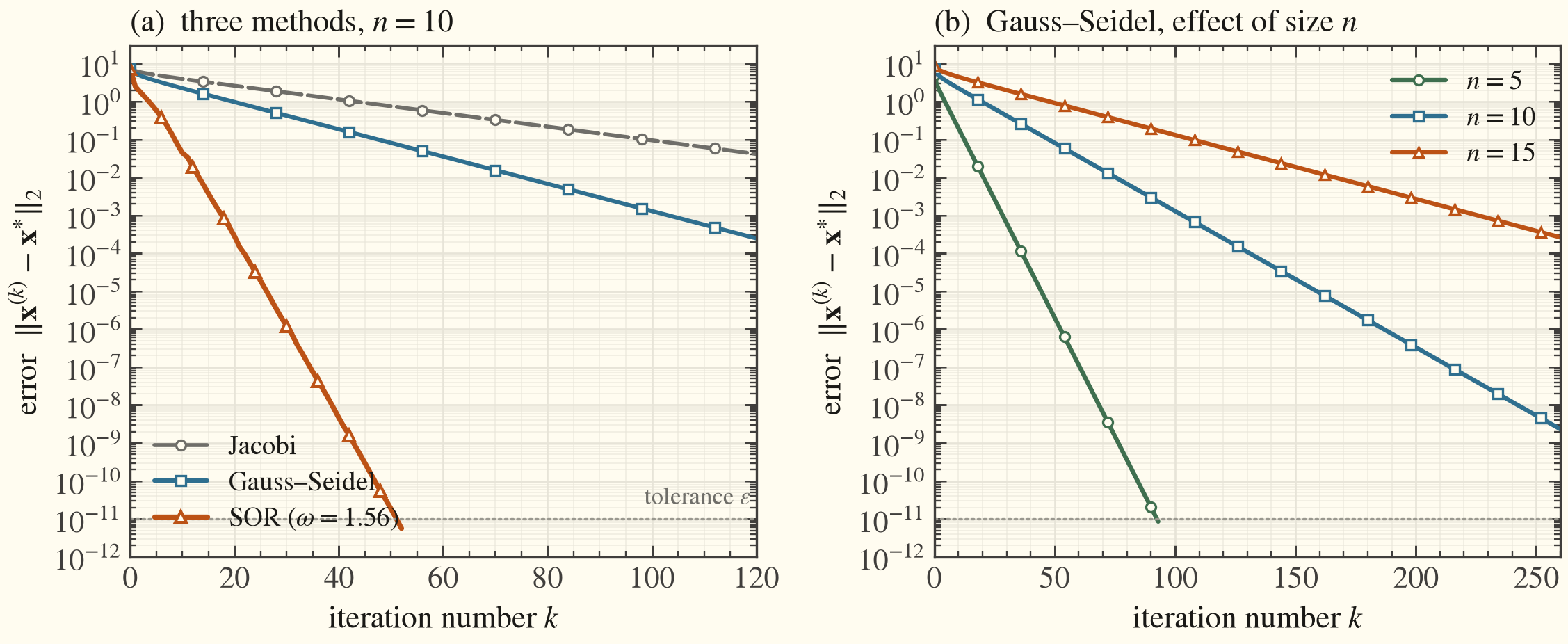 Error versus iteration count (left) for the three methods, and (right) the effect of system size on Gauss-Seidel
The take-away mirrors the discussion in the course: Gauss-Seidel roughly halves the iteration count of Jacobi, while a well-chosen over-relaxation factor reduces it by another order of magnitude. For the very large systems produced by realistic two- and three-dimensional discretizations, this difference is decisive, and stationary methods are in turn often used as smoothers or preconditioners within more advanced multigrid and Krylov solvers.