An excerpt from the lecture notes of a course I taught entitled Constitutive Modelling in Geomechanics. Because the response of a soil cannot depend on the orientation of the axes we happen to choose, constitutive models are written in terms of stress invariants: scalar combinations of the stress components that take the same value in every coordinate system. This note develops those invariants, the split of stress into hydrostatic and deviatoric parts, and the derived measures that appear throughout geomechanics. A compression-positive sign convention is used, as is customary in soil mechanics.
The Stress Tensor and its Invariants
The state of stress at a point is described by the symmetric second-order tensor \(\sigma_{ij}\). Its three principal stresses \(\sigma_1 \geq \sigma_2 \geq \sigma_3\) are the roots of the characteristic equation
\[\sigma^3 - I_1 \sigma^2 + I_2 \sigma - I_3 = 0\]whose coefficients are the three principal invariants of the stress tensor,
\[I_1 = \sigma_{kk} = \sigma_1 + \sigma_2 + \sigma_3\] \[I_2 = \tfrac{1}{2}\left( \sigma_{ii}\sigma_{jj} - \sigma_{ij}\sigma_{ij} \right) = \sigma_1\sigma_2 + \sigma_2\sigma_3 + \sigma_3\sigma_1\] \[I_3 = \det(\sigma_{ij}) = \sigma_1 \sigma_2 \sigma_3\]Being invariants, \(I_1\), \(I_2\) and \(I_3\) are unchanged by any rotation of the coordinate axes.
Hydrostatic and Deviatoric Decomposition
It is convenient to separate the part of the stress that changes volume from the part that distorts the material. The mean stress is
\[p = \frac{1}{3} I_1 = \frac{1}{3}\left( \sigma_1 + \sigma_2 + \sigma_3 \right)\]and the stress tensor is split into a hydrostatic (spherical) part and a deviatoric part \(s_{ij}\),
\[\sigma_{ij} = p\, \delta_{ij} + s_{ij}, \qquad s_{ij} = \sigma_{ij} - p\, \delta_{ij}\]The deviatoric tensor carries the shearing, or distortional, part of the stress. Its first invariant vanishes by construction, \(J_1 = s_{kk} = 0\), and the remaining invariants are
\[J_2 = \tfrac{1}{2} s_{ij} s_{ij} = \frac{1}{6}\left[ (\sigma_1-\sigma_2)^2 + (\sigma_2-\sigma_3)^2 + (\sigma_3-\sigma_1)^2 \right]\] \[J_3 = \det(s_{ij})\]The second deviatoric invariant \(J_2\) is the single most important stress measure in plasticity. It is usually expressed through the deviatoric stress (also called the equivalent or von Mises stress),
\[q = \sqrt{3 J_2}\]which reduces to \(q = \sigma_1 - \sigma_3\) in a triaxial test where \(\sigma_2 = \sigma_3\). Together, \(p\) and \(q\) form the coordinates of the triaxial stress space in which most soil models are formulated.
Octahedral Stresses and the Lode Angle
The same information appears in the octahedral stresses, defined on the plane whose normal is equally inclined to the three principal directions,
\[\sigma_{\mathrm{oct}} = \frac{1}{3} I_1 = p, \qquad \tau_{\mathrm{oct}} = \sqrt{\tfrac{2}{3} J_2} = \frac{1}{3}\sqrt{(\sigma_1-\sigma_2)^2 + (\sigma_2-\sigma_3)^2 + (\sigma_3-\sigma_1)^2}\]so that \(q = \tfrac{3}{\sqrt{2}}\, \tau_{\mathrm{oct}}\). A third quantity is needed to fix the position on the octahedral plane: the Lode angle \(\theta\), which measures the relative magnitude of the intermediate principal stress and is defined through
\[\cos 3\theta = \frac{3\sqrt{3}}{2} \frac{J_3}{J_2^{3/2}}\]The triplet \((p, q, \theta)\), mean stress, deviatoric stress, and Lode angle, completely describes the stress state up to orientation, and is the coordinate system in which yield and failure criteria are most naturally drawn.
A Worked Example
Consider a stress state with principal stresses \(\sigma_1 = 120\), \(\sigma_2 = 60\) and \(\sigma_3 = 30\) kPa. The mean stress is
\[p = \frac{120 + 60 + 30}{3} = 70~\mathrm{kPa}\]so that the principal deviatoric stresses are \(s_1 = 50\), \(s_2 = -10\) and \(s_3 = -40\) kPa. The second deviatoric invariant and the deviatoric stress follow as
\[J_2 = \tfrac{1}{6}\left[ 60^2 + 30^2 + 90^2 \right] = 2100~\mathrm{kPa}^2, \qquad q = \sqrt{3 \times 2100} = 79.4~\mathrm{kPa}\]and the octahedral shear stress is \(\tau_{\mathrm{oct}} = \sqrt{2 \times 2100 / 3} = 37.4\) kPa. The three Mohr circles for this state are shown below; the largest has radius \(\tau_{\max} = (\sigma_1 - \sigma_3)/2 = 45\) kPa, and the mean stress \(p\) locates the centroid of the principal stresses on the normal-stress axis.
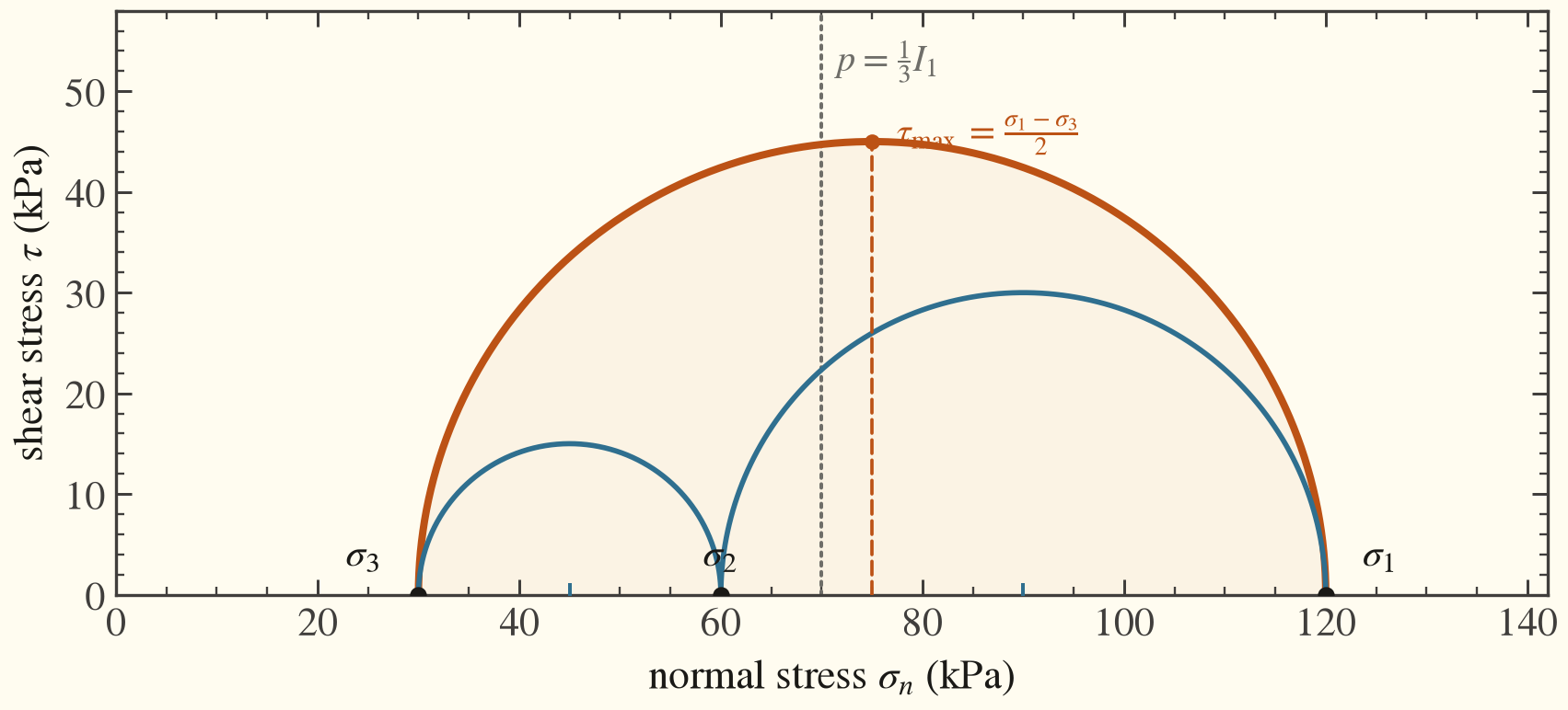 The three Mohr circles for the principal stresses, with the maximum shear stress and mean stress indicated
Computing the Invariants
For a general stress tensor the invariants and principal stresses are obtained directly from the matrix. The short routine below returns the quantities defined above.
import numpy as np

def stress_invariants(sigma):
    I1 = np.trace(sigma)
    I2 = 0.5 * (np.trace(sigma) ** 2 - np.trace(sigma @ sigma))
    I3 = np.linalg.det(sigma)
    p = I1 / 3.0
    s = sigma - p * np.eye(3)
    J2 = 0.5 * np.tensordot(s, s)
    J3 = np.linalg.det(s)
    q = np.sqrt(3.0 * J2)
    sig_principal = np.sort(np.linalg.eigvalsh(sigma))[::-1]
    lode = np.degrees(np.arccos(
        np.clip(1.5 * np.sqrt(3.0) * J3 / J2 ** 1.5, -1.0, 1.0)) / 3.0)
    return dict(I1=I1, I2=I2, I3=I3, p=p, q=q, J2=J2, J3=J3,
                principal=sig_principal, lode_deg=lode)

sigma = np.array([[100.0, 30.0,  0.0],
                  [ 30.0, 50.0, 20.0],
                  [  0.0, 20.0, 40.0]])
for key, val in stress_invariants(sigma).items():
    print(key, np.round(val, 3))
For the tensor above this gives \(I_1 = 190\) kPa, \(p = 63.3\) kPa and \(q = 83.7\) kPa, principal stresses \((115.1,\, 55.5,\, 19.4)\) kPa, and a Lode angle of \(22.0^\circ\). These invariants, not the individual stress components, are what a constitutive model sees, and they are the building blocks for the yield and failure criteria discussed in the next note.